



With advances in AGI advancing at a rapid pace, the ability to start talking with the latest models in real time will be at the forefront of integrating AGI solutions into everyday life.
In this post, I’ll be discussing audio processing, Whisper, and share my notebook so you can follow along or try it out for yourself!
Hopefully by the end of this post you’ll be able to answer:
-
What are audio signals and how do they work?
-
How are audio signals processed into frequencies?
-
What is the MEL spectrogram?
-
What is Whisper?
Audio
Recording sound
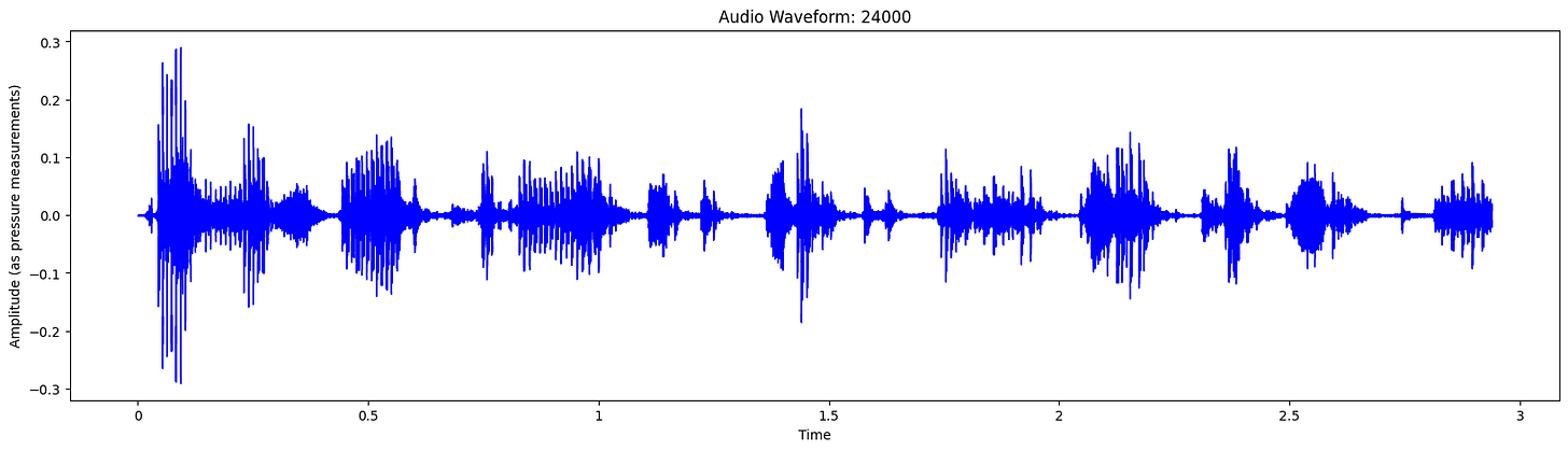
We’ll be using the above audio signal for this discussion. The way to think about audio is as a waveform, specifically oscillations in pressure (compression and refraction) of the air. See Figure 1.
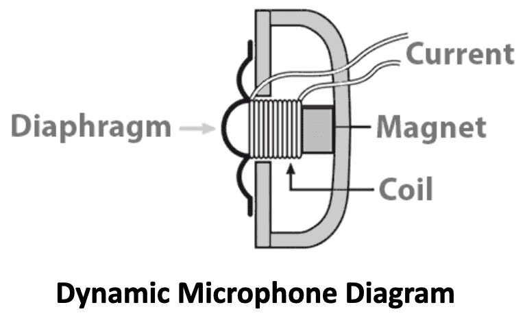
These waveforms are recorded using microphones that use a small diaphragm (see figure 2). Negative values typically indicate refraction where the diaphragm is pulled out and positive values indicate compression where the diaphragm is pushed in. Thus, using this setup we can measure our audiowave signal!
Audio samples, the number values we get from the microphone, can be represented in many different ways but a common way is with floating point numbers where -1 represents some minimum negative value, 0 is no sound pressure, and 1 represents some maximum positive value. The larger the number the louder the sound.
In order to get a good reading of an audio signal like the one above, we need to sample values of the microphone at some frequency, like 16,000 hz. What this means is that for every second of audio we take 16,000 audio samples, which means 16,000 values between [-1, 1]. A frequency like 16,000 is typically called the sampling rate, CDs (I know I know no one uses them anymore) have a sampling rate of about 44,100 hz. Plotting the above audio signal at a sampling rate of 24,000 hz (the rate of my microphone) we get the following curve.
Audio signals to frequencies
There is an important property in signal processing that comes from something called the Fourier transform, which for now can be thought of as a method for decomposing our signal into an infinite sum of real valued cosine waves and imaginary sine waves.
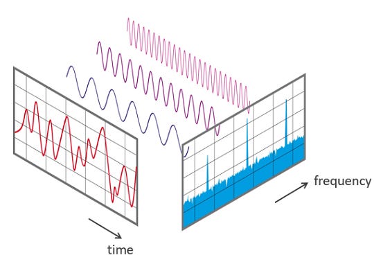
Similar to how reading a recipe can tell us all the ingredients in a smoothie the Fourier transform can tell us all ‘ingredient’ signals at various amplitudes that when added together give us our audio output ‘smoothie’.
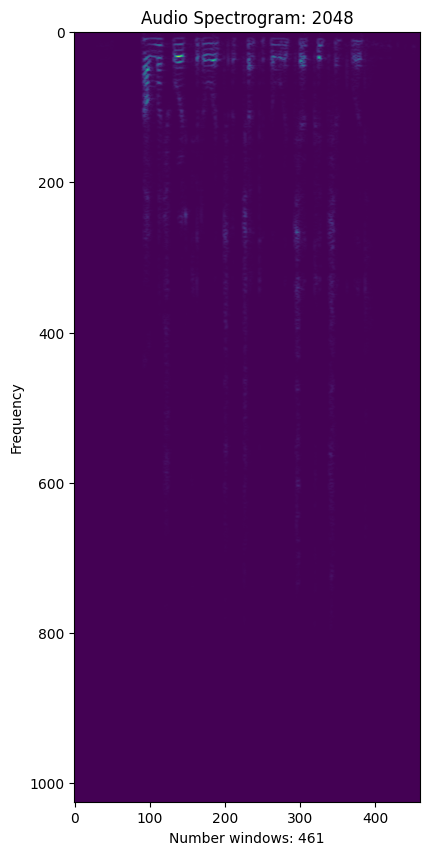
To convert from audio signals to frequencies we use the Fast Fourier Transform (FFT) (for the discrete case). Specifically, we take a sliding window of time and compute all those frequencies in that bin of time. For instance, if we have a 10 second audio clip, our sliding window is 0.1 seconds and our stride is also 0.1 seconds then we’ll produce 100 smaller audio clips and run them through the FFT, giving us a list of frequencies at different intensities (ie some frequencies might be louder than others). If you plot an image where on the x-axis you have each of these smaller audio clips represented as a single point and on the y-axis you have the values of the various frequencies you get a spectrogram.
Human perception and Mel frequencies
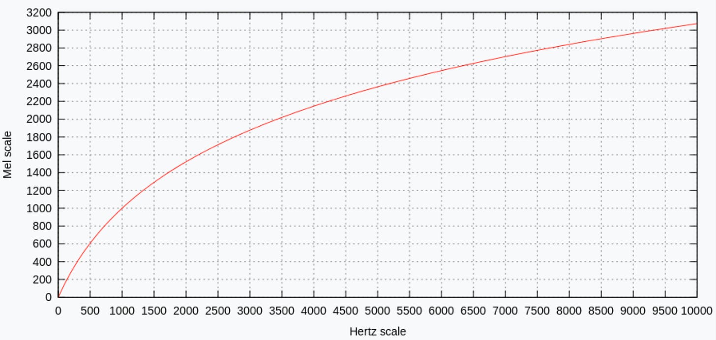
In the 1970s, psychologists studying human audio perception made a curious discovery: that as humans listen to higher frequencies we have a harder time distinguishing between them, meaning humans have an easier time distinguishing between lower frequencies compare to higher frequencies. This is due to humans percieving logarithmically. One analogy is holding a 10 pound weight and shifting to 20 pounds which would feel like adding 10 lbs. But 100 lbs to 110 lbs doesn’t feel like adding 10 lbs. This percept we have with weight changes we also have with sound changes and after psychologists collected data from many participants on just-noticeable differences in pitch (frequency) a logarithmic perception of sound emerged as shown in Figure 6. On the x-axis is the actual frequency and on the y-axis the predicted perceived value. Thus was born the Mel scale.
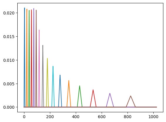
This observation lead to handpicking certain perceptible “bins” for humans, where certain ranges of lower and higher frequencies are grouped together. The way to think about it is, humans have more trouble distinguishing higher frequencies so as the frequency goes up just make the bin wider (see Figure 7). These are called Mel filters, we take each one of them and slide them across time to generate weighted sums.
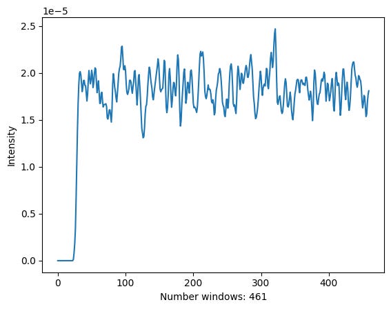
If we take the last Mel bin for higher frequencies (the brown triangle in Figure 7) and slide it over our frequency spectrogram (Figure 5) we’ll get a single number across time which looks like this.
Doing this for all 80 Mel filters and plotting the Mel spectrogram again yields figure 9.
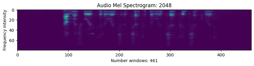
Now we’re almost finished with our audio processing (and getting the inputs used for the whisper model). The last processing step is to convert the signals to DB space meaning we take the log of all these signals. Doing so gives us Figure 10.
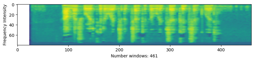
And volia! The Log-Mel spectrogram that’s used as input to the Whisper model.
Whisper Model
Overview
Multitask training
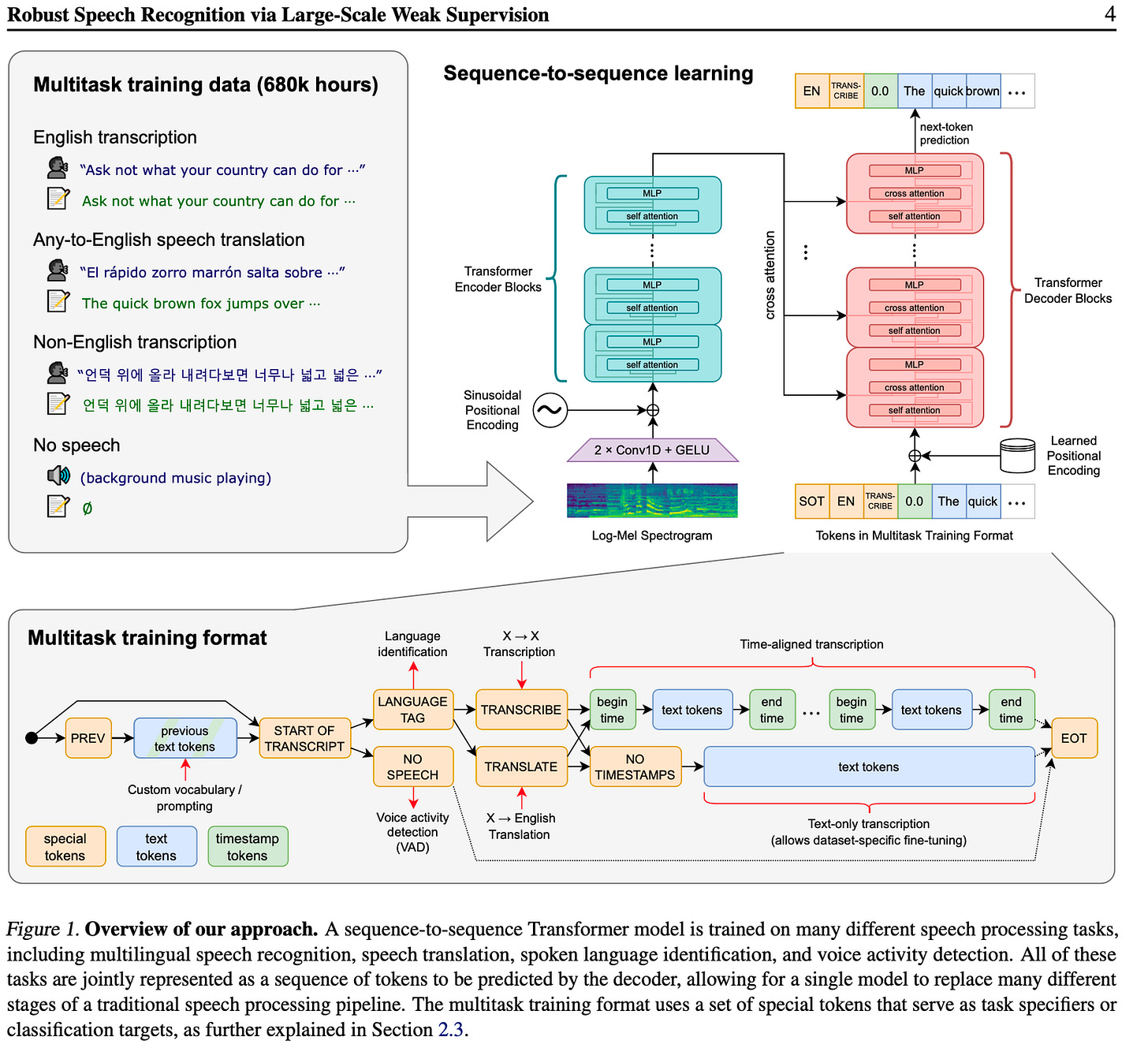
The significant contribution that made Whisper an incredible Speech to Text (STT) model was the authors focused on using pre-training on the decoder. The decoder is trained to be a multitask predictor (transcription, translation, voice activity detection, etc.). As shown in Figure 11, using the previous text or previous prediction as a conditional input (the start begins with startoftranscript (SOT)) they predict the language being spoken or no speech. Once the language is predicted the task is specified with a special token. Then if desired the model is asked to predict time boxes around each of the words otherwise it just returns the text (the text ends with endoftranscript (EOT)). This setup is what distinguished Whisper from other automatic speech recognition models; Whisper is able to transcribe, translate, and condition on the previous prediction with significantly high fidelity.
Data
Their data used audio-text pairs they found on the internet they collected a corpus of multilingual multimodal data, filtering out any machine generated audio-text pairs. All audio files are also broken up into 30 second segments.
Model
And finally their model is the standard encoder-decoder Transformer architecture in the Attention is all you need paper save they convolve the Log-Mel spectrogram along each of the 80 channels by 3 into a 512 latent space.
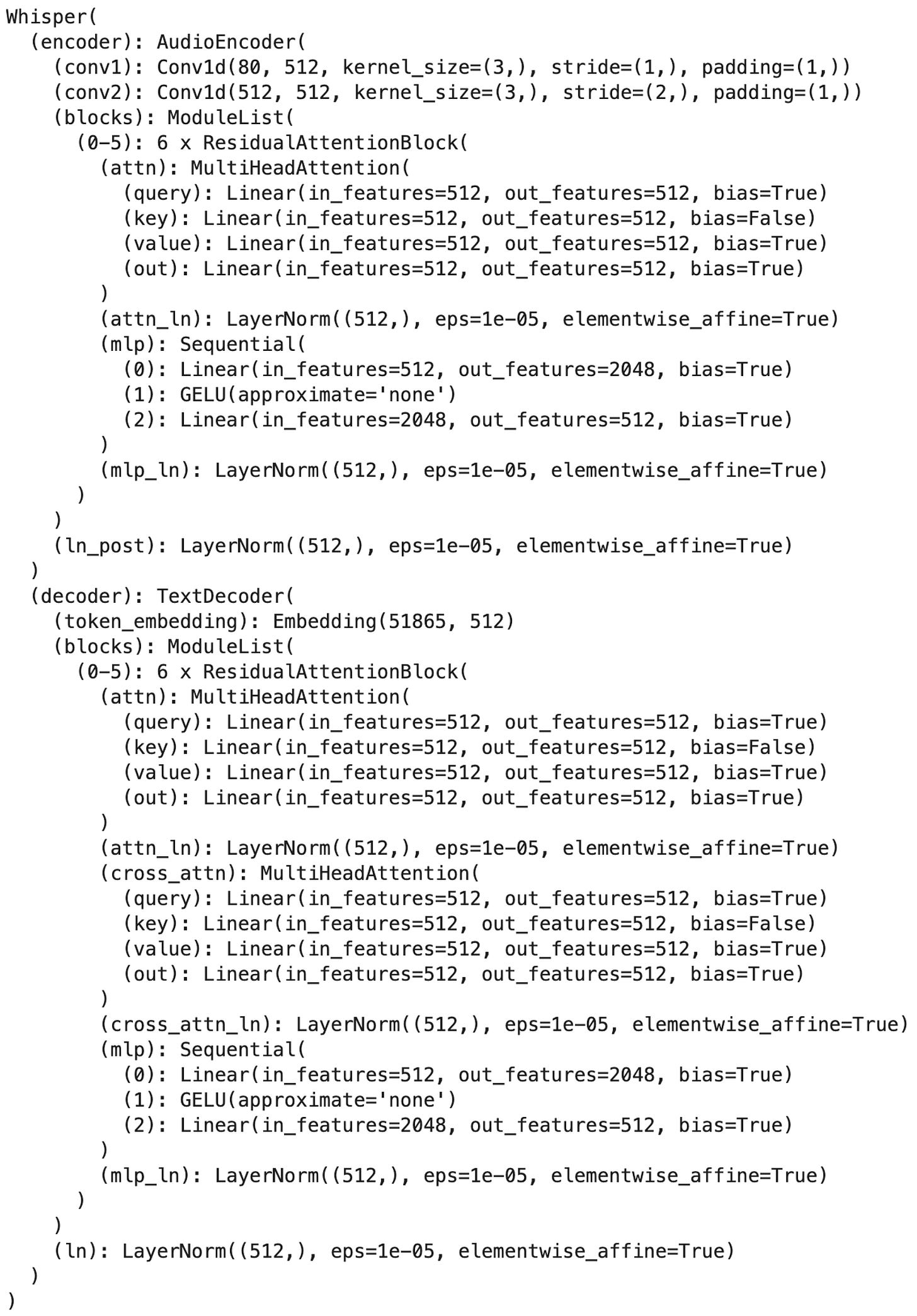
Finally, using whisper let’s try transcribing our audio signal
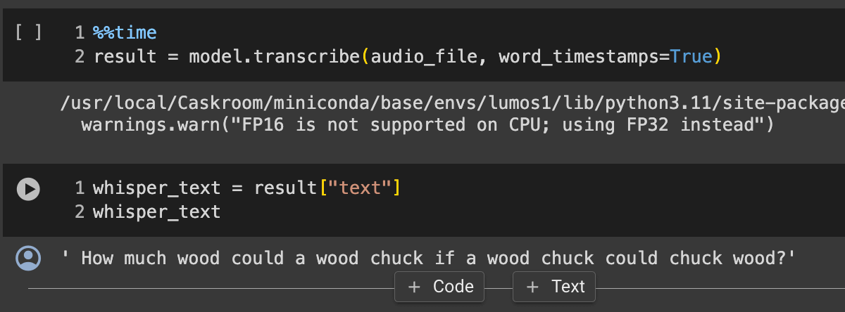
So we notice that the transcription is not bad but omits a “chuck” and doesn’t link woodchuck but overall impressive!
Conclusion
In this blog we walk through how an audio signal is measured and converted into a digital signal, how that digital signal is converted into frequencies, how those frequencies are processed into a Log-Mel spectrogram, and how that Log-Mel spectrogram is consumed by the Whisper architecture. We then discussed Whisper contributions including how it focused on pretraining strategies for the decoder—specifically configuring and training multiple tasks in a single decoder, the data that Whisper was trained on, and the model architecture.
As always, I hope you enjoyed this post! If you want to play around with audio processing and try Whisper for yourself checkout my notebook here!
Fun Facts
-
A microphone transforms an analog signal to a digital one; waveforms are sampled rapidly at different frequencies and measured as voltages that ultimately fall between [-1, 1] (in our representation).
-
Whisper stands for Web-scale Supervised Pretraining for Speech Recognition.
References