



Overview
This article is a deeply technical continuation of our previous high level discussion of Reinforcement Learning. Now we begin to get a bit more into the weeds.
In this article, we discus Markov Decision Process transition kernels vs structural / state-equation representations of the same dynamics. The main takeway is that a transition kernel Pr[s’ | s, a] and a noise driven equation s’ = f(s,a,w) can generate the same one-step stochastic dynamics at various levels of abstraction. We’ll aside on causal models and then we’ll work through an example connecting these concepts.
Reminder: What is RL ?
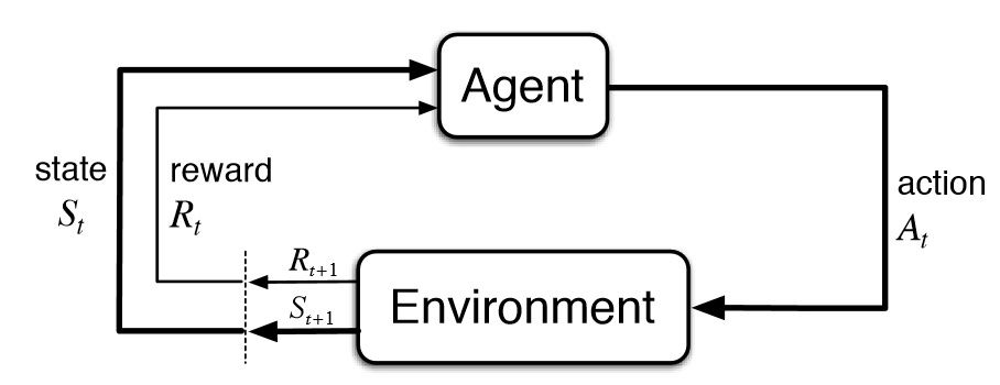
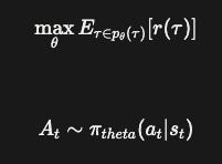
As a reminder Reinforcement Learning (RL) is a type of learning procedure where an agent learns how to act in an evolving environment with unknown world dynamics. The agent’s “policy” is what takes actions in this world effecting the environment’s state and leading to the next state. How an agent learns is based on the reward feedback. We try to maximize the expected reward over all sequences of actions (trajectories) an agent takes given some policy.
MDP vs SEM transitions
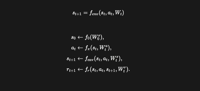
Like in the previous post, usually reinforcement learning is presented with Markov Decision Processes (MDPs). Uncertainty is hidden behind the notion of probability sometimes obscuring where the randomness actually comes from. See the environment evolution probabilities below.
Cue sequential equation models, which explicitly model a sequence of state actions over some trajectory deterministically with a quantifiable exogenous random variable. The notation is a bit different but translating this looks like
where W_t is a random variable that models irreducible noise. Inside the function, f_env, we can model something deterministic.
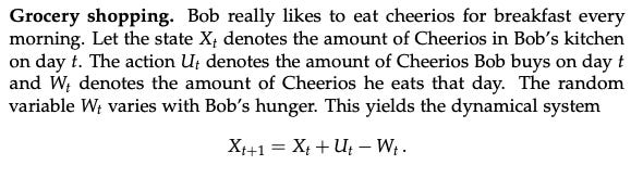
An example from “Patterns, Predictions, Actions” is Grocery shopping (X_t is the state, U_t is the action).
The cool part about this is the notation is distributional equivalent subject to the conditions. Essentially

Distributional equivalence is weaker than causal equivalence
At a high level, an SEM becomes causal when we define how every variable in the system is generated; formally when we explicitly make each variable an endogenous or exogenous variable. When we constructed Bob’s SEM we made assumptions about W_t that may or may not be true which made the system probabilistic. Bob’s true number of cheerios eaten is an exogenous variable; a variable that we model probabilistically but in reality could have some other hidden set of dynamics. For instance, Bob’s hunger depends on the energy he used so a true causal relationship b/w hunger would be energy consumption and modeled differently. Compare this to the amount of Cherrios remaining; here, X_{t+1} is an endogenous variable b/c it’s completely defined by it’s parents: once we know the amount of Cherrios we already have, the number of Cherrios purchased, and bob’s hunger we can immediately determine the next amount of Cherrios. [1]
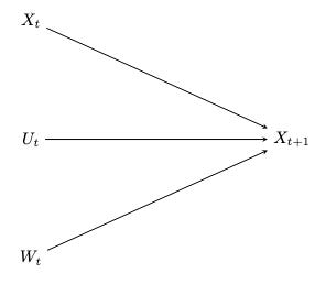
If for example we instead wanted to model bob’s hunger as something that effects how many Cherrios he consumes
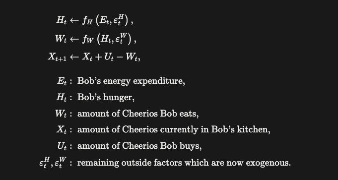
In this model setup W_t is now endogenous since it’s fully defined by f_w.
What this means generally
Causal models let us do interventions. Since we’ve fully modeled the system we can do(”w_t = eat lots of cheerios”) and observe the system. For our use case, it’s enough to say that our SEM below evolves into a SCM when we have explicit assignments of each variable not just equality.
Uniting these two concepts
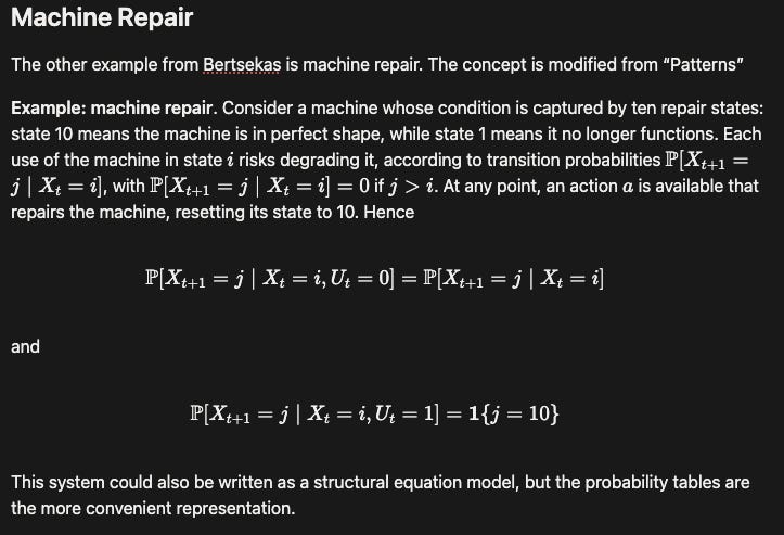
Below we walk through an example that takes an MDP’s dynamical system for machine repair and we translate it into it’s SEM form. This is mostly an exercise but shows how deeply connected the two concepts are.
Discrete SEM
But as a proof of concept let’s translate this to a sequential decision making process. Let
if j <= i o.w. j > i => 0 which means that the model can only decay not suddenly improve. To convert this into a SEM we need a deterministic function with an exogenous random variable.
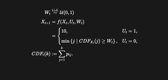
The CDF here is piecewise summing b/c the states of the machine have discrete conditional probabilities. For instance, in state 5 all states at or below 5 have some probability that sum to 1. Our uniform distribution and W_t represents a probability and we need to map that probability to the value, in this case the machine state. This is the role of the inverse CDF and what we constructed when the action is 0 (do nothing).
Continuous PDF
Now let’s extend this a bit to continuous states. Let’s imagine that the machine was continuously decaying rather than just a discrete set. What’s a good way to model this? One way is to make this linear meaning that the probability of decaying close to 0 is less likely than decaying closer to 1. Note that we’ve extended machine states from [1, 10] to [0, 10].
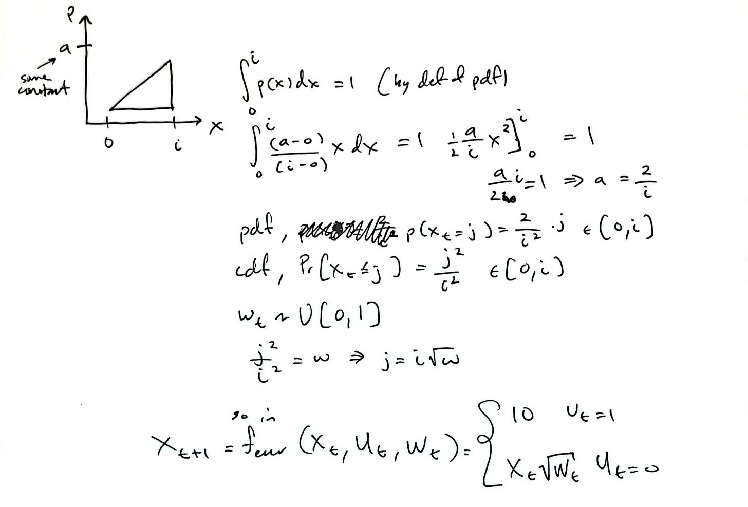
So now we need to sample randomly along the uniform dist [0, 1] and map it to the state of the machine and since the U[0,1] represents the possible outputs of the CDF using the inverse CDF gives us the machine state that could’ve given us that probability.
Why RL courses usually start with MDPs
Mostly convenience. Structural equations explicitly model how a system evolves. For physics based problems like a falling ball or control based problems like the bicycle model SEM representations can more naturally model known dynamics and explicit disturbances W_t are better understood. However as we discussed, MDPs are more abstract and just probabilistically model transitions between states without an understanding of the mechanism that produces each transition. This lets RL courses introduce policies, value functions, and Bellman equations without a detailed physical model of the environment. Dynamics are not ignored and model based algorithms learn or use it but the difference can remain at the level of transition probabilities.
Conclusion
Takeaway: when approaching problems that solve RL problems, it can be useful to consider both notations as some are more natural than others. For environments where certain assumptions can make our life easier we can use SEMs while when these assumptions is too much of a simplification we can stay abstract with MDPs. Consider both though the next time you’re looking at the dynamics.
Appendix
- [1] Different kinds of uncertainty: Aleatoric uncertainty which is inherent randomness of the environment that cannot be reduced by more data or more exploration (measurement / observational differences, data collection changes, etc.). Epistemic uncertainty is when the agent is reducible and shrinks as more data is collected. For instance the transition dynamics are not known, or the model’s own policy. A caveat is that the boundary b/w the two is still a modeling choice. A coin flip is aleatoric if we just observe flips but if we modeled the coin with perfect physics and initial conditions it’s deterministic up to measurement error. If more data reduces a kind of uncertainty it’s epistemic else it’s aleatoric.