



Recall
Reinforcement learning (RL) is a sequential decision making process where an agent takes actions in the environment with some dynamics and receives rewards. Typically the dynamics of the environment Pr[S’ | S, A] are unknown, but in today’s article we’ll walk through a toy RL problem with known dynamics to build intuition on what RL is even solving.
This article assumes a bit of familiarity with Q functions and briefly touches on interesting properties & principles that will be relevant for our toy example.
Cue Q-functions
Recall the setup for sequential decision making processes
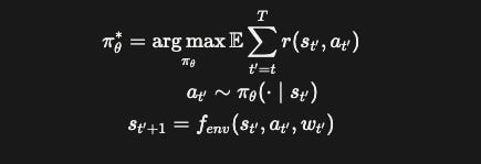
Q-functions are the expected reward for some trajectory starting at initial state s_t, a_t up to some future timestep T.

The above equation means if we start at s_t, force the first action to be a_t and then follow the policy \pi for all subsequent steps for all possible trajectories we get some average reward. The Q-function under some policy, \pi is not necessarily optimal. The way to imagine this is if on our way to starbucks we stop by the gym which is in the other direction. It’s a policy that perhaps gets us to starbucks but it’s not fastest route. Which brings us into an optimal Q-function under an optimal policy \pi^*.

This definition is more nuanced since it’s saying after we take the first action we search over all possible actions and pick the action that maximizes our expected reward. The optimal policy for such a function is a bit circular but essentially it’s the action that maximizes the expected reward at every time step (assuming the last timestep is T). In our starbucks example, instead of the gym we go to the park which is the fastest way to get to starbucks. We can define our optimal policy in terms of Q function (despite being a bit circular).

The beauty of this optimal policy is that bellman equation falls out directly from the principle of optimality. If the optimal path from point A to point B passes through point C then the optimal path from A→ C and C → B must also be optimal. For instance if on my walk to starbucks from my house and I pass through the park then the optimal route from the park to starbucks must be the optimal path I take when I go from my house to starbucks since we went through the park. If there was another optimal path say around the park then walking to through the park to starbucks was never optimal to begin with and hence we have a contradiction! We represent this idea with the bellman equation: the optimal path of an existing state & action at time is the reward at the current step + the optimal path state, action pair for the next step.

This concept, the bellman equation, principle of optimality, is the basis for all dynamic programming problems: if a complex problem can be broken down recursively into a set of simpler but similar subproblems to some base case then by induction we can solve the original problem. If I can solve the path from starbucks to the park, then solve for the path from the park to starbucks I have the optimal path!
And with those ides let’s jump into our toy problem.
Gridworld
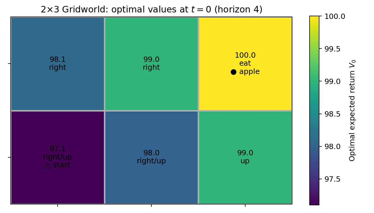
Suppose that we have a 2 x 3 grid where we have ego ( a triangle) trying to eat an apple (the dot). In this setup we show how we’d find the tabular solution to this toy example with Q functions in this dynamic program.
+---------+---------+---------+
| 0       | 1       | 2   ●   |
+---------+---------+---------+
| 3   △   | 4       | 5       |
+---------+---------+---------+
What are the states?
-
ego location: . There are 6 places ego can be.
-
visited: a binary string of 1’s x 0’s. There are 6 bits required for marking each state, giving 2**6 different “visited” states.
-
This gives us the following cardinality of our state space

What are the actions?
- 5 total actions

What are the dynamics of the world?
One of the key parts, we’re constructing the dynamics in this example. w_t is some random noise that makes this environment probablisitic.
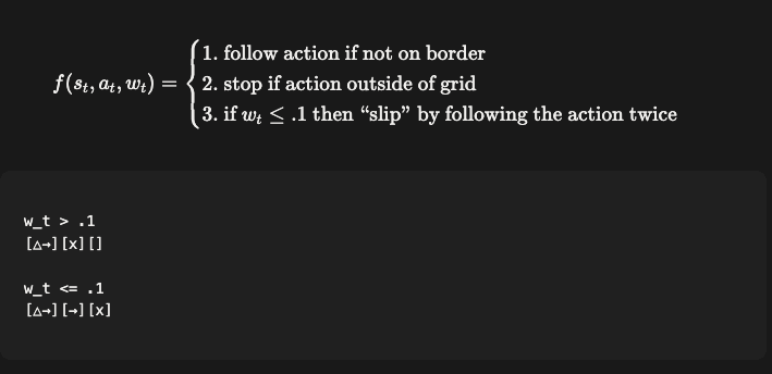
Above we show an example of slippage (where ego might go past the desired location). If the slippage is up it’ll just degenerate to a single action up.
What is the reward function?

Construct the transition table
B/c the size of the state, actions pairs is constrained and because we have the dynamics of the environment we can fully map the transition table of the environment at each times step. Note that below that the left hand side contains all ego state, all visited state, and all actions. 384 * 5 = 1920 rows. The column is all of the states = 384.
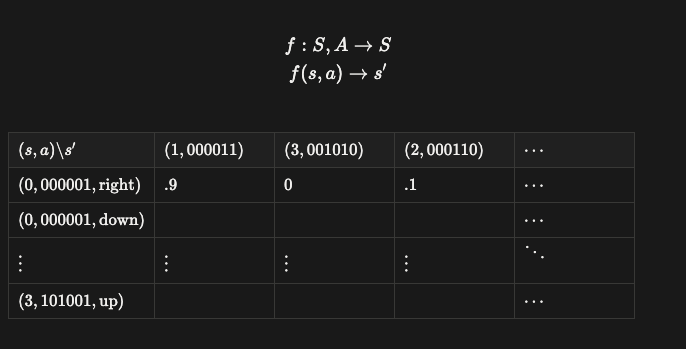
Notice it's a very sparse matrix!
Compute the Q table as a dynamic program
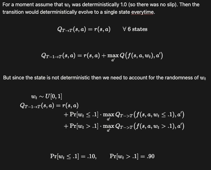
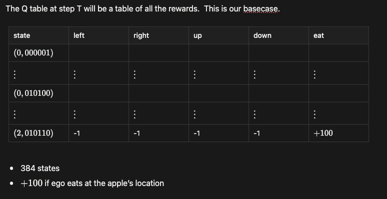
We start with this and build a Q table for every time step using the above equation at every state, action pair!
The actual algorithm:
-
Let’s codify what this update step would look like & construct the update step


-
First take the maximum over the next action:, this gives us the optimal value for each state.
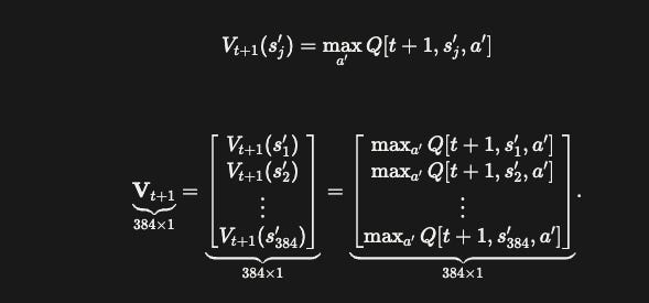
-
Flatten the transition table so that each row is one (s, a) pair: The rows represent all of the possible state, action pairs and the columns represent all the possible states that the environment can evolve into.
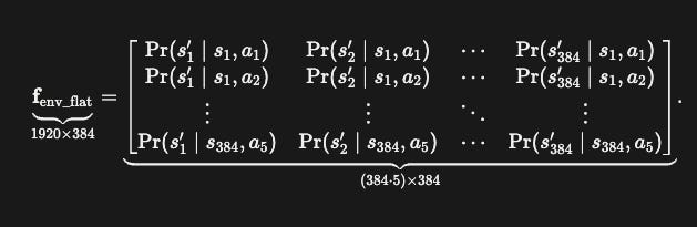
-
Multiply the flattened transition matrix by the vector of state values from the t+1 timestep. We essentially sum the probability of transitioning to every other state given our current state action pair.
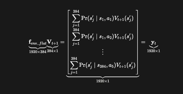
-
A single row of the matrix multiplication is
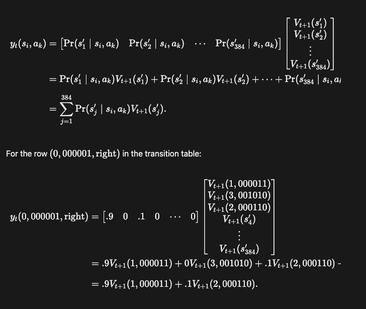
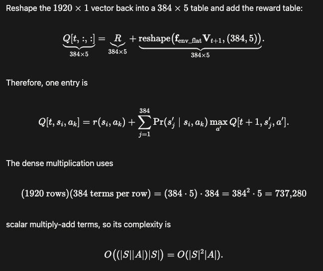
And that’s it! For our gridworld example we can explicitly solve for the optimal solution and with modern packages like numpy this can be done very quickly.
Conclusion
With known probability transitions solving for a sequential decision making process becomes a dynamic program, and we can use the principle of optimality with our basecase to inductively solve a more complex problem. We discussed some interesting properties of a general Q function and an optimal Q function with an optimal policy and we walked through a toy Gridworld Tabular MDP example with known dynamics that helps contextualize how RL under the hood woks.
To play with the example we showed in code checkout this gist.
For extra material chec
kout Karpathy’s Reinforcejs which has a similar Gridworld or try coding / vibecoding it yourself!